de_analysis and de_design perform differential analysis of measured
lipids that are associated with a sample group (annotation). de_analysis
accepts a list of contrasts, while de_design allows users to define a
design matrix, useful for complex experimental designs or for adjusting
possible confounding variables.
de_analysis(data, ..., measure = "Area", group_col = NULL)

de_design(data, design, ..., coef = NULL, measure = "Area")

significant_molecules(de.results, p.cutoff = 0.05, logFC.cutoff = 1)

plot_results_volcano(de.results, show.labels = TRUE)
Arguments
- data
LipidomicsExperiment object, should be normalized and log2 transformed.
- ...
Expressions, or character strings which can be parsed to expressions, specifying contrasts. These are passed to
limma::makeContrasts.- measure
Which measure to use as intensity, usually Area (default).
- group_col
Name of the column containing sample groups. If not provided, defaults to first sample annotation column.
- design
Design matrix generated from
model.matrix(), or a design formula.- coef
Column number or column name specifying which coefficient of the linear model is of interest.
- de.results
Output of
de_analysis().- p.cutoff
Significance threshold. Default is
0.05.- logFC.cutoff
Cutoff limit for log2 fold change. Default is
1. Ignored in multi-group (ANOVA-style) comparisons.- show.labels
Whether labels should be displayed for significant lipids. Default is
TRUE.
Value
TopTable as returned by limma package
significant_molecules returns a character vector with names of
significantly differentially changed lipids.
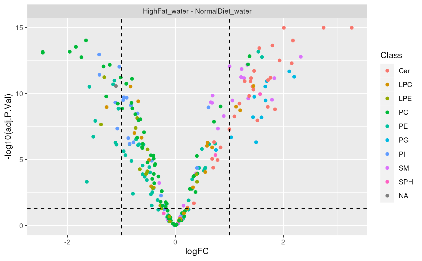
plot_results_volcano returns a ggplot object.
Functions
significant_molecules(): gets a list of significantly changed lipids for each contrast.plot_results_volcano(): plots a volcano chart for differential analysis results.
Examples
# type ?normalize_pqn to see how to normalize and log2-transform your data
data(data_normalized)

# Specifying contrasts
de_results <- de_analysis(
  data_normalized,
  HighFat_water - NormalDiet_water,
  measure = "Area"
)
# Using formula
de_results_formula <- de_design(
  data = data_normalized,
  design = ~group,
  coef = "groupHighFat_water",
  measure = "Area"
)

# Using design matrix
design <- model.matrix(~group, data = colData(data_normalized))
de_results_design <- de_design(
  data = data_normalized,
  design = design,
  coef = "groupHighFat_water",
  measure = "Area"
)
significant_molecules(de_results)
#> $`HighFat_water - NormalDiet_water`
#>  [1] PE 32:1         PE 32:2         PE 34:2         PE 34:3
#>  [5] PE 36:5         PE 38:2         PE(O-34:2)      PE(O-38:4)
#>  [9] PE(P-32:0)      PE(P-34:1)      PE(P-34:2)      PE(P-38:3)
#> [13] PG 16:0/18:1    PG 16:1/16:0    PG 18:0/16:0    PG 18:1/18:0
#> [17] PG 18:1/18:1    PG 18:2/16:0    PG 18:2/18:0    PG 18:2/18:1
#> [21] PG 20:4/16:0    PG 20:4/16:1    PI 32:2         PI 32:3
#> [25] PI 34:1p        PI 34:2         PI 34:3         PI 36:3
#> [29] Sa1P d 18:0     SM 18:1/16:2    SM 18:1/18:0    SM 18:1/18:1
#> [33] SM 18:1/20:0    SM 18:1/20:2    SM 18:1/22:3    SM 18:1/22:4
#> [37] SM 18:1/22:5    SM d18:0/18:0   SM d18:0/20:0   Cer d18:0/C16:0
#> [41] Cer d18:0/C18:0 Cer d18:0/C20:0 Cer d18:0/C22:0 Cer d18:0/C24:0
#> [45] Cer d18:0/C24:1 Cer d18:0/C24:2 Cer d18:1/C16:0 Cer d18:1/C16:1
#> [49] Cer d18:1/C18:0 Cer d18:1/C18:1 Cer d18:1/C20:0 Cer d18:1/C20:1
#> [53] Cer d18:1/C20:2 Cer d18:1/C22:0 Cer d18:1/C22:1 Cer d18:1/C22:2
#> [57] Cer d18:1/C22:3 Cer d18:1/C22:5 Cer d18:1/C22:6 Cer d18:1/C24:1
#> [61] Cer d18:1/C26:0 Cer d18:2/C20:0 PC 36:5         PC 36:6
#> [65] PC 40:2         PC 40:8         LPC 20:0        LPC 20:4
#> [69] LPC 22:0        LPC 26:0        LPE 20:0        LPE 20:5
#> [73] PC(O-34:2)      PC(O-34:3)      PC(O-38:2)      PC(O-40:1)
#> [77] PC(P-34:1)      PC(P-34:2)      PC(P-34:3)      PC(P-36:5)
#> [81] PC(P-38:0)      PC(P-38:1)      PC(P-40:0)
#> 277 Levels: PE 32:0 PE 32:1 PE 32:2 PE 34:1 PE 34:1 NEG PE 34:2 ... PC(P-40:6)
#>
plot_results_volcano(de_results, show.labels = FALSE)