Data mining using lipidr
Ahmed Mohamed
Precision & Systems Biomedicine, QIMR Berghofer, Australia2023-06-08
Source:vignettes/examples/mw_integration.Rmd
mw_integration.RmdIntroduction
Through integration with Metabolomics Workbench API,
lipidr allows users, to quickly explore public lipidomics
experiments. lipidr provides an easy way to re-analyze and
visualize these datasets.
Loading libraries
First, we load lipidr using library
command. For this vignette we will enable interactive graphics plotting
by calling use_interactive_graphics().
Explore Metabolomics Workbench lipidomics datasets
Users can search all Metabolomics Workbench studies using any
relevant keyword. A list of all studies matching the keyword will be
returned as a table (data.frame).
list_mw_studies(keyword = "lipid")Download datasets
Datasets can be easily downloaded and parsed into
LipidomicsExperiment object using lipidr
function fetch_mw_study() by supplying a
study_id. The example shown in this vignette is from
ST001111 link.
The dataset contains positive and negative MS data for untargeted
lipidomics from different breast cancer tissues.
d = fetch_mw_study("ST001111")

d
## class: LipidomicsExperiment
## dim: 777 118
## metadata(4): summarized dimnames summarized dimnames
## assays(1): Area
## rownames(777): CE 16:0 [M+NH4]+ CE 16:1 [M+NH4]+ ... PS 44:6
## (22:1(13Z)/22:5(4Z.7Z.10Z.13Z.16Z)) [M-H]- PS 46:5
## (22:5(4Z.7Z.10Z.13Z.16Z)/24:0) [M-H]-
## rowData names(22): filename Molecule ... total_cs Class
## colnames(118): 1 2 ... 117 118
## colData names(4): SampleType Race Stage Tumor.TypeNote the warning that some molecules were not parsed because their names did not follow the supported patterns. We can examine these molecules, remove them from the dataset or change their names, if desired.
# list non_parsed molecules
non_parsed_molecules(d)
## [1] "SB N-(15Z-tetracosenoyl)-sphing-4-enine (d18:1/24:1)"
## [2] "SB N-(9Z-octadecenoyl)-sphinganine (d18:0/18:1)"
## [3] "SB N-(docosanoyl)-sphing-4-enine (d18:1/22:0)"
## [4] "SB N-(eicosanoyl)-sphing-4-enine (d18:1/20:0)"
## [5] "SB N-(hexadecanoyl)-sphing-4-enine (d18:1/16:0)"
## [6] "SB N-(octadecanoyl)-sphing-4-enine (d18:1/18:0)"
## [7] "SB N-(octadecanoyl)-sphinganine (d18:0/18:0)"
## [8] "SB N-(tetracosanoyl)-sphing-4-enine (d18:1/24:0)"
# All of them are Ceramides, written with full chemical name
# We can replace the first part with "Cer" using RegEx
non_parsed <- non_parsed_molecules(d)
new_names <- sub("^.* \\(", "Cer (", non_parsed)
d <- update_molecule_names(d, old = non_parsed, new = new_names)

# We can check once again to make sure all molecules were parsed correctly
non_parsed_molecules(d)
## character(0)We can have a look at the clinical data, which was conveniently
extracted from Metabolomics Workbench by lipidr.
colData(d)Next, we tell lipidr that our dataset is normalized and
logged.
d <- set_logged(d, "Area", TRUE)
d <- set_normalized(d, "Area", TRUE)
Quality control
We look at total ion concentration (TIC) and distribution (boxplot) for each sample.
plot_samples(d, "tic")
plot_samples(d, "boxplot")Although the TIC plot looks similar for all samples, we can spot two
outlier samples with significantly large dispersion (samples
42 and 18). We will keep the samples for now,
but we may want to consider checking closely.
Because there is no QC samples or technical replicates in this
dataset, we cannot assess the %CV of molecules. Also, there is no need
to summarize_transitions in untargeted datasets.
PCA
mvaresults = mva(d, measure="Area", method="PCA")
plot_mva(mvaresults, color_by="SampleType", components = c(1,2))
We can see mild separation between benign and cancer samples, but not
between cancer and metastasis. We can also spot the sample outlier
samples that should consider removing. The low variance explained by
PC1 and PC2 (cumulative displayed in the plot
as R2X) indicate highly variable lipid profiles in these
clinical samples.
Univariate Analysis
Two group comparison
For simple analysis, we can compare cancer vs benign and cancer vs metastasis. From PCA plot, we can expect very little difference between cancer and metastasis.
two_group <- de_analysis(d, Cancer-Benign, Cancer-Metastasis)
plot_results_volcano(two_group)
By quickly looking at the volcano plots, we can confirm the minute difference between cancer and metastatic samples. A fairly large difference is observed between cancer and benign samples, with PCs and PGs up-regulated and CLs and TGs down-regulated in cancer tissues.
Multi-group comparison
Instead of two-group comparison, we might be interested in lipids are
differentially expressed in any group. We can perform ANOVA-style
multi-group comparison using de_design function, which
allows users to provide a custom design matrix.
de_design is extremely helpful in complex experimental
designs, where several factors should be accounted for in the
analysis.
In this example, we will use cancer stage as our grouping variable. In our dataset, we can see samples with Stages I-IV. Using ANOVA-style analysis, we will identify all lipid molecules likely to be different among cancer stages.
multi_group <- de_design(d, ~ Stage)Here we used the formula tilde to define our predictor
variables. ~ Stage formula indicates that we are interested
in features (lipid molecules) that are associated with
Stage.
significant_molecules(multi_group)## named list()Surprisingly, Cancer Stage does not appear to affect lipid molecules profiled in this experiment.
Factorial analysis
In complex experimental designs and clinical samples, we may need to
correct for confounding variables. This is done simply by adding the
variable to the formula in de_design. For example, below,
we are interested in Cancer effect while correcting for Race
effect.
factorial_de <- de_design(d, ~ Race + SampleType, coef = "SampleTypeCancer")
significant_molecules(factorial_de)
## $SampleTypeCancer
## [1] "CE 18:1" "CE 18:2"
## [3] "CE 20:4" "DG (14:0/16:0/0:0)"
## [5] "DG (14:0/16:1/0:0)" "DG (14:1/16:0/0:0)"
## [7] "DG (12:0/18:2/0:0)" "DG (15:0/16:0/0:0)"
## [9] "DG (17:0/14:0/0:0)" "DG (14:0/18:1/0:0)"
## [11] "DG (16:1/16:0/0:0)" "DG (14:0/18:2/0:0)"
## [13] "DG (15:0/18:1/0:0)" "DG (16:0/18:2/0:0)"
## [15] "DG (16:1/18:1/0:0)" "DG (16:0/18:3/0:0)"
## [17] "DG (16:1/18:2/0:0)" "DG (16:1/18:3/0:0)"
## [19] "DG (16:0/20:3/0:0)" "DG (18:1/18:2/0:0)"
## [21] "DG (18:2/18:3/0:0)" "DG (16:0/22:0/0:0)"
## [23] "DG (18:2/22:1/0:0)" "DG (22:2/18:1/0:0)"
## [25] "DG (16:0/26:0/0:0)" "DG (18:1/26:0/0:0)"
## [27] "DG (18:1/26:1/0:0)" "lysoPC 15:0"
## [29] "lysoPC 17:1" "lysoPC 21:0"
## [31] "lysoPC 24:0" "PA (7:0/16:1)"
## [33] "PA (9:0/26:1)" "PC (13:0/16:1)"
## [35] "PC (14:0/15:1)" "PC (26:1/3:0)"
## [37] "PC (7:0/22:1)" "PC (14:1/16:0)"
## [39] "PC (11:0/21:0)" "PC (14:0/18:0)"
## [41] "PC (15:0/17:0)" "PC (16:0/16:0)"
## [43] "PC (18:0/14:0)" "PC (6:0/26:0)"
## [45] "PC (12:0/20:1)" "PC (14:0/18:1)"
## [47] "PC (16:0/16:1)" "PC (14:0/18:2)"
## [49] "PC (15:1/17:1)" "PC (17:2/15:0)"
## [51] "PC (11:0/22:0)" "PC (16:0/17:0)"
## [53] "PC (23:0/10:0)" "PC (7:0/26:2)"
## [55] "PC (16:0/18:1)" "PC (12:0/22:2)"
## [57] "PC (16:0/18:2)" "PC (16:1/18:1)"
## [59] "PC (16:0/18:3)" "PC (16:1/18:2)"
## [61] "PC (17:0/18:1)" "PC (13:0/22:5)"
## [63] "PC (15:0/20:5)" "PC (15:1/20:4)"
## [65] "PC (15:0/21:0)" "PC (18:0/18:0)"
## [67] "PC (10:0/26:1)" "PC (14:0/22:1)"
## [69] "PC (18:0/18:1)" "PC (16:0/20:2)"
## [71] "PC (18:0/18:2)" "PC (18:1/18:1)"
## [73] "PC (16:0/20:3)" "PC (16:1/20:2)"
## [75] "PC (12:0/24:4)" "PC (24:4/12:0)"
## [77] "PC (18:2/18:3)" "PC (11:0/26:1)"
## [79] "PC (16:1/21:0)" "PC (18:1/19:0)"
## [81] "PC (26:1/11:0)" "PC (12:0/26:1)"
## [83] "PC (14:1/24:0)" "PC (15:1/23:0)"
## [85] "PC (18:0/20:1)" "PC (18:0/20:1)"
## [87] "PC (18:1/20:0)" "PC (21:0/17:1)"
## [89] "PC (22:1/16:0)" "PC (16:0/22:2)"
## [91] "PC (18:0/20:2)" "PC (18:1/20:1)"
## [93] "PC (18:2/20:0)" "PC (20:2/18:0)"
## [95] "PC (24:1/14:1)" "PC (18:0/20:3)"
## [97] "PC (18:2/20:1)" "PC (18:0/20:5)"
## [99] "PC (18:1/20:4)" "PC (18:2/20:3)"
## [101] "PC (22:5/16:0)" "PC (16:1/22:6)"
## [103] "PC (18:4/20:4)" "PC (18:1/21:0)"
## [105] "PC (17:0/22:2)" "PC (17:1/22:6)"
## [107] "PC (17:2/22:5)" "PC (15:0/25:0)"
## [109] "PC (17:0/23:0)" "PC (24:1/16:0)"
## [111] "PC (25:0/15:1)" "PC (14:0/26:2)"
## [113] "PC (16:1/24:1)" "PC (17:2/23:0)"
## [115] "PC (24:1/16:1)" "PC (18:1/22:2)"
## [117] "PC (18:2/22:1)" "PC (18:3/22:0)"
## [119] "PC (20:0/20:3)" "PC (18:2/22:2)"
## [121] "PC (20:2/20:2)" "PC (18:1/22:5)"
## [123] "PC (20:2/20:4)" "PC (20:3/20:3)"
## [125] "PC (18:1/22:6)" "PC (18:2/22:5)"
## [127] "PC (20:2/20:5)" "PC (20:3/20:4)"
## [129] "PC (18:2/23:0)" "PC (19:0/23:0)"
## [131] "PC (16:0/26:2)" "PC (16:1/26:1)"
## [133] "PC (18:1/24:1)" "PC (18:2/24:0)"
## [135] "PC (20:1/22:1)" "PC (20:2/22:0)"
## [137] "PC (18:2/24:1)" "PC (18:4/24:0)"
## [139] "PC (20:4/22:1)" "PC (18:2/24:4)"
## [141] "PC (20:0/22:6)" "PC (20:4/22:2)"
## [143] "PC (18:2/26:2)" "PC (18:2/26:2)"
## [145] "PC (20:0/24:4)" "PC (20:3/24:1)"
## [147] "PC (22:2/22:2)" "plasmenylPC (16:0/14:0)"
## [149] "plasmenylPC (16:0/19:0)" "plasmenylPC (20:0/17:0)"
## [151] "plasmenylPC (18:0/22:2)" "TG (12:0/12:0/16:0)"
## [153] "TG (12:0/14:0/16:0)" "TG (12:0/12:0/18:1)"
## [155] "TG (12:0/16:1/16:0)" "TG (12:0/16:1/16:1)"
## [157] "TG (14:0/16:0/16:0)" "TG (14:0/16:0/16:0)"
## [159] "TG (14:0/16:0/16:1)" "TG (14:0/16:0/16:1)"
## [161] "TG (12:0/18:1/16:1)" "TG (14:0/16:0/18:1)"
## [163] "TG (14:0/16:0/18:1)" "TG (14:0/16:1/18:1)"
## [165] "TG (14:1/16:1/18:1)" "TG (16:0/16:1/17:1)"
## [167] "TG (16:0/16:0/18:0)" "TG (16:0/16:1/18:1)"
## [169] "TG (16:0/16:1/18:1)" "TG (16:0/16:1/18:2)"
## [171] "TG (16:0/17:0/18:2)" "TG (16:0/16:0/20:0)"
## [173] "TG (16:0/18:0/18:1)" "TG (17:0/17:0/18:1)"
## [175] "TG (16:0/18:1/18:1)" "TG (16:0/18:2/18:2)"
## [177] "TG (16:0/16:1/20:4)" "TG (16:0/18:2/18:3)"
## [179] "TG (16:0/18:2/18:3)" "TG (16:1/18:2/18:3)"
## [181] "TG (16:1/18:2/18:3)" "TG (16:1/18:3/18:3)"
## [183] "TG (16:0/17:0/20:0)" "TG (17:0/18:0/18:1)"
## [185] "TG (17:0/18:0/18:2)" "TG (17:0/18:1/18:1)"
## [187] "TG (17:0/18:1/18:2)" "TG (17:1/18:1/18:2)"
## [189] "TG (17:1/18:2/18:3)" "TG (17:2/18:2/18:3)"
## [191] "TG (16:0/18:0/20:0)" "TG (16:0/18:1/20:0)"
## [193] "TG (18:0/18:0/18:1)" "TG (16:0/18:0/20:1)"
## [195] "TG (16:0/18:1/20:0)" "TG (16:0/18:1/20:1)"
## [197] "TG (18:0/18:1/18:1)" "TG (16:0/18:1/20:1)"
## [199] "TG (16:0/18:1/20:3)" "TG (16:0/18:2/20:3)"
## [201] "TG (18:1/18:2/18:2)" "TG (16:0/16:0/22:6)"
## [203] "TG (16:0/18:2/20:4)" "TG (16:0/16:1/22:6)"
## [205] "TG (18:2/18:2/18:3)" "TG (18:2/18:2/18:3)"
## [207] "TG (18:2/18:3/18:3)" "TG (17:0/18:1/20:0)"
## [209] "TG (18:0/18:2/19:0)" "TG (18:1/18:1/19:0)"
## [211] "TG (18:1/18:2/19:0)" "TG (16:0/18:0/22:1)"
## [213] "TG (17:0/19:0/20:1)" "TG (16:0/18:0/22:2)"
## [215] "TG (16:1/20:0/20:1)" "TG (18:0/18:2/20:0)"
## [217] "TG (16:0/20:1/20:2)" "TG (18:1/18:1/20:1)"
## [219] "TG (18:1/18:2/20:1)" "TG (16:0/18:2/22:6)"
## [221] "TG (18:1/18:2/20:5)" "TG (18:2/18:3/20:3)"
## [223] "TG (16:0/18:3/22:6)" "TG (18:0/18:1/21:0)"
## [225] "TG (18:1/19:0/20:1)" "TG (18:0/19:0/20:3)"
## [227] "TG (17:0/18:1/22:4)" "TG (16:0/20:5/22:6)"
## [229] "TG (16:1/20:4/22:6)" "TG (18:2/20:4/20:5)"
## [231] "TG (18:1/20:3/20:4)" "TG (17:0/20:1/22:1)"
## [233] "TG (18:2/20:3/22:4)" "TG (18:1/22:4/22:5)"
## [235] "TG (18:2/22:4/22:5)" "TG (18:0/22:0/22:4)"
## [237] "TG (18:1/22:1/22:2)" "TG (18:1/22:0/22:4)"
## [239] "TG (18:1/22:1/22:5)" "TG (20:1/20:4/22:4)"
## [241] "CL (14:0/18:1/16:0/18:1)" "CL (16:0/16:1/16:0/18:1)"
## [243] "CL (16:0/18:1/16:1/16:0)" "CL (18:1/14:0/18:1/16:0)"
## [245] "CL (16:0/18:1/16:1/18:0)" "CL (18:0/16:0/18:2/16:0)"
## [247] "CL (16:0/16:1/18:0/18:2)" "CL (16:0/16:1/18:1/18:2)"
## [249] "CL (16:1/16:1/18:2/18:1)" "CL (16:1/18:0/18:2/18:1)"
## [251] "CL (18:1/16:0/18:2/18:2)" "CL (18:0/16:0/18:0/20:0)"
## [253] "CL (18:3/14:0/20:3/20:4)" "CL (18:1/18:0/20:1/16:0)"
## [255] "CL (16:0/20:2/18:1/18:0)" "CL (18:0/18:1/18:2/18:0)"
## [257] "CL (18:0/18:2/18:1/18:0)" "CL (16:0/22:5/16:1/20:4)"
## [259] "CL (16:1/22:5/20:4/16:0)" "CL (16:1/22:0/18:1/18:2)"
## [261] "CL (18:2/18:1/20:1/18:0)" "CL (18:1/18:1/18:1/20:3)"
## [263] "CL (18:1/18:2/20:2/18:1)" "CL (18:1/18:1/18:2/20:3)"
## [265] "CL (18:1/18:2/20:2/18:2)" "CL (18:1/20:2/18:2/18:2)"
## [267] "CL (18:2/18:1/20:3/18:2)" "CL (18:2/18:2/18:2/20:2)"
## [269] "CL (18:0/20:4/18:2/18:3)" "CL (18:2/20:3/18:3/18:1)"
## [271] "CL (16:0/18:0/20:4/22:6)" "CL (16:0/22:6/18:0/20:4)"
## [273] "CL (18:0/22:6/20:4/16:0)" "CL (16:0/18:1/22:6/20:4)"
## [275] "CL (18:2/18:2/20:4/20:3)" "CL (18:3/20:3/20:4/18:2)"
## [277] "CL (18:2/18:1/20:1/20:2)" "CL (18:1/18:2/20:3/20:2)"
## [279] "CL (18:2/18:1/20:2/20:3)" "CL (18:0/16:0/22:5/20:4)"
## [281] "CL (18:0/20:4/18:1/20:4)" "CL (16:0/22:6/22:5/18:0)"
## [283] "CL (18:1/20:4/18:2/22:6)" "CL (20:0/20:0/20:1/18:1)"
## [285] "CL (20:1/20:0/20:1/18:1)" "CL (20:0/18:1/20:1/20:2)"
## [287] "CL (20:0/20:0/18:2/20:2)" "CL (20:0/20:2/18:2/20:0)"
## [289] "CL (18:0/20:1/20:2/20:3)" "CL (20:1/18:2/20:1/20:2)"
## [291] "CL (18:0/22:6/18:2/22:6)" "CL (18:0/20:0/22:5/22:6)"
## [293] "CL (18:0/20:0/22:6/22:5)" "CL (18:0/22:5/20:0/22:6)"
## [295] "CL (20:1/18:0/22:5/22:6)" "Cer (d18:1/24:1)"
## [297] "Cer (d18:1/22:0)" "Cer (d18:1/20:0)"
## [299] "Cer (d18:1/16:0)" "PA (17:0/17:0)"
## [301] "PA (18:1/20:1)" "PC (2:0/22:2)"
## [303] "PC (2:0/26:2)" "PC (12:0/17:0)"
## [305] "PC (14:0/16:0)" "PC (16:0/17:0)"
## [307] "PC (16:0/18:1)" "PC (17:2/17:0)"
## [309] "PE (14:0/18:1)" "PE (16:0/16:1)"
## [311] "PE (14:0/18:2)" "PE (16:1/17:0)"
## [313] "PE (17:0/18:0)" "PE (17:1/18:1)"
## [315] "PE (17:0/19:0)" "PE (18:0/18:2)"
## [317] "PE (16:0/20:5)" "PE (17:0/20:3)"
## [319] "PE (18:0/20:0)" "PE (18:1/20:2)"
## [321] "PE (16:0/22:5)" "PE (16:0/24:1)"
## [323] "PE (18:2/22:0)" "PE (18:1/22:2)"
## [325] "PE (20:1/20:2)" "PE (20:1/20:3)"
## [327] "PE (18:0/22:5)" "PE (18:1/22:4)"
## [329] "PE (18:0/24:1)" "PE (18:1/24:0)"
## [331] "PE (20:1/22:1)" "PE (20:3/22:0)"
## [333] "PE (18:0/24:4)" "PE (18:1/24:4)"
## [335] "PE (20:4/22:1)" "PE (20:1/22:6)"
## [337] "PE (20:2/22:6)" "PE (20:3/24:0)"
## [339] "PE (18:2/26:2)" "PE (20:5/24:0)"
## [341] "PG (17:0/16:0)" "PG (16:1/18:2)"
## [343] "PG (18:1/20:4)" "PG (18:2/20:3)"
## [345] "PG (18:3/20:4)" "PG (18:0/22:5)"
## [347] "PG (18:1/22:5)" "PG (18:2/22:4)"
## [349] "PG (18:1/22:6)" "PG (20:3/20:4)"
## [351] "PG (20:3/22:4)" "PG (20:4/22:5)"
## [353] "PI (18:0/20:1)" "PI (20:0/20:4)"
## [355] "PI (20:1/20:4)" "plasmenylPE (16:0/18:2)"
## [357] "plasmenylPE (20:0/22:6)" "PS (15:1/18:1)"
## [359] "PS (17:0/17:0)" "PS (16:1/18:1)"
## [361] "PS (17:0/19:0)" "PS (16:0/20:3)"
## [363] "PS (18:0/18:3)" "PS (16:0/20:5)"
## [365] "PS (18:1/20:0)" "PS (18:1/20:2)"
## [367] "PS (18:1/20:4)" "PS (19:0/20:4)"
## [369] "PS (20:5/20:5)" "PS (20:0/20:3)"
## [371] "PS (18:0/22:4)" "PS (20:1/20:3)"
## [373] "PS (18:0/22:5)" "PS (18:1/22:4)"
## [375] "PS (20:1/22:4)" "PS (22:0/22:6)"
## [377] "PS (22:1/22:5)"
plot_results_volcano(factorial_de)In this case, we are seeing similar pattern as the two-group comparison, which indicates a small Race effect.
Users interested in creating more complex design matrices are referred to Limma User Guide and edgeR tutorial.
Multivariate analysis
Orthogonal multivariate analysis
Supervised multivariate analyses, such as OPLS and OPLS-DA can be performed to determine which lipids are associated with a group (y-variable) of interest. In this example we use “Diet” as grouping, and display the results in a scores plot.
mvaresults = mva(d, method = "OPLS-DA", group_col = "SampleType", groups=c("Benign", "Cancer"))
plot_mva(mvaresults, color_by="SampleType")
We can also plot the loadings and display important lipids contributing to the separation between different (Diet) groups.
plot_mva_loadings(mvaresults, color_by="Class", top.n=10)Alternatively, we can extract top N lipids along with their annotations.
top_lipids(mvaresults, top.n=10)Supervised multivariate analysis with continuous response variable
OPLS-DA can only be applied to in two-group comparison settings. In some cases, we might be interested in a lipid molecules ….
In this example, we will format Cancer Stage as a numeric vector.
stage <- d$Stage
stage[stage == "I"] <- 1
stage[stage == "II"] <- 2
stage[stage == "III"] <- 3
stage[stage == "IV"] <- 4
stage <- as.numeric(stage)
stage
## [1] 2 2 3 3 1 2 4 3 NA 2 2 NA 1 3 3 3 2 3 2 3 2 1 3 2 2
## [26] 2 1 2 1 NA 2 2 3 2 2 1 3 2 2 2 1 3 1 3 3 3 2 2 2 3
## [51] 2 1 3 2 1 NA 2 2 1 2 1 2 1 3 2 2 2 1 NA 1 1 1 1 2 1
## [76] 1 2 2 NA 4 1 1 1 2 2 1 3 2 2 3 2 2 1 NA 1 2 3 2 2 4
## [101] 3 2 2 2 2 1 1 2 2 2 3 3 2 2 2 2We can see stage contains missing values. We should
filter them out first.
d_filtered <- d[, !is.na(stage)]
stage <- stage[!is.na(stage)]

mvaresults = mva(d_filtered, method = "OPLS", group_col = stage )
plot_mva(mvaresults)
use_interactive_graphics(FALSE)
plot_mva_loadings(mvaresults, color_by="Class", top.n=10)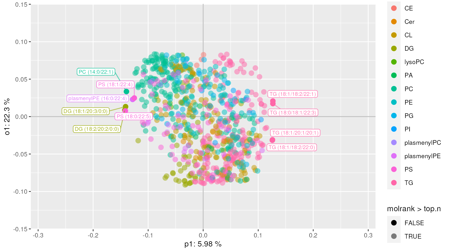
Enrichment analysis
enrich_results = lsea(two_group, rank.by = "logFC")
significant_lipidsets(enrich_results)
## $`Cancer - Benign`
## [1] "Class_PC" "Class_TG" "total_cl_40" "total_cl_54" "total_cl_56"
## [6] "Class_DG" "total_cl_52" "total_cl_53" "total_cl_38" "total_cl_29"
## [11] "total_cl_66" "Class_CL" "total_cl_58" "total_cl_34" "total_cl_76"
## [16] "total_cl_62" "total_cs_9" "Class_PG" "Class_CE" "total_cs_7"
## [21] "total_cl_32"
##
## $`Cancer - Metastasis`
## [1] "Class_TG" "Class_PC" "total_cl_56" "total_cl_58" "Class_PS"
## [6] "Class_PG" "total_cl_55" "Class_CE" "total_cl_70" "Class_PE"
## [11] "total_cl_42" "total_cl_57" "total_cs_1" "total_cl_59" "total_cl_29"
## [16] "total_cl_18"Visualization of enrichment analysis results. The enriched lipid classes are highlighted.
plot_enrichment(two_group, significant_lipidsets(enrich_results), annotation="class")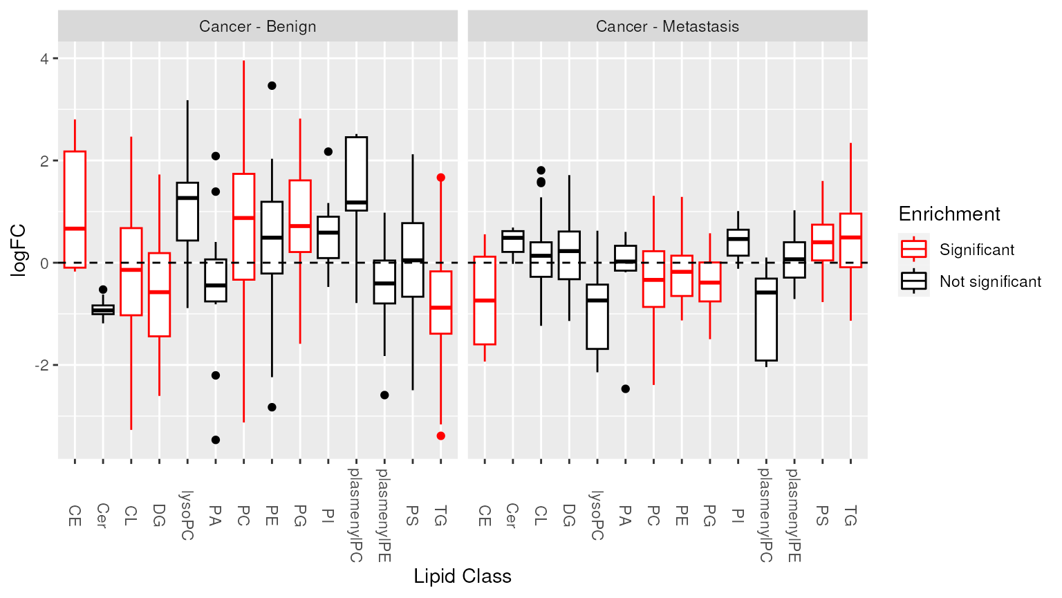
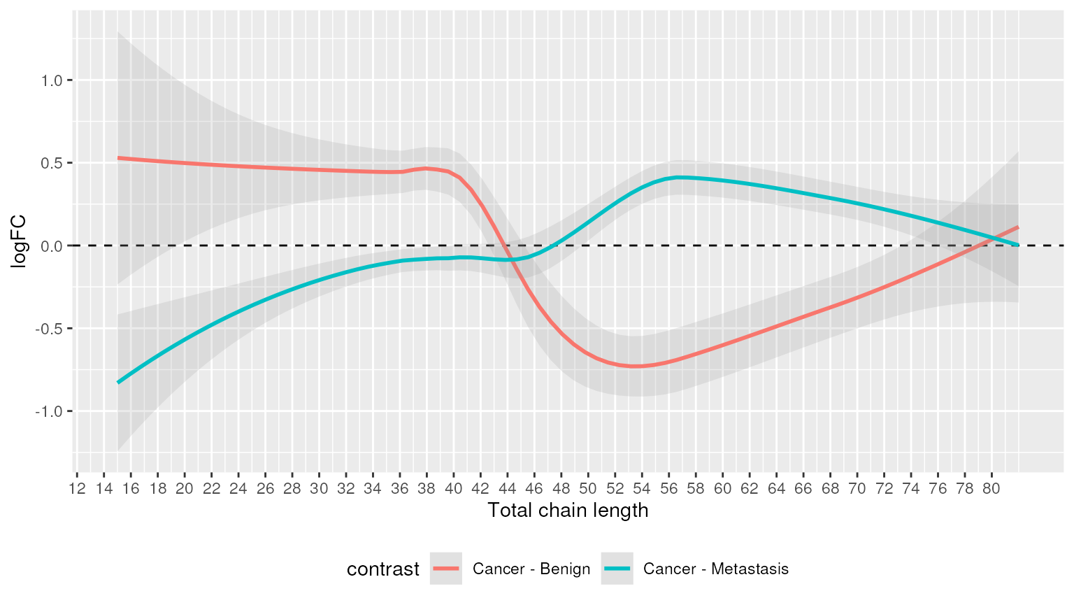
Alternatively, we can highlight chain lengths that were significantly enriched.
plot_enrichment(two_group, significant_lipidsets(enrich_results), annotation="length")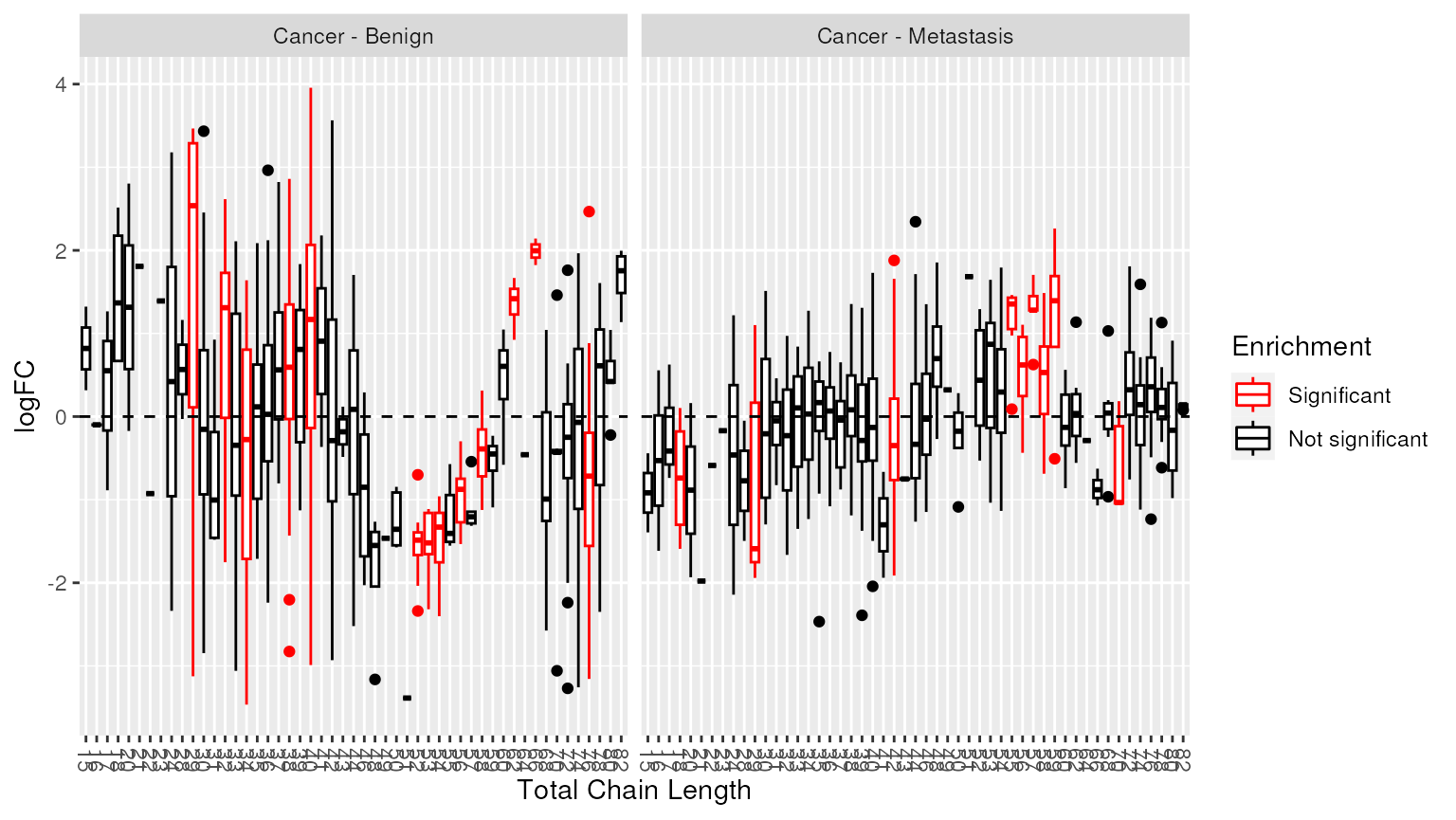
Session information
## R version 4.3.0 (2023-04-21)
## Platform: x86_64-pc-linux-gnu (64-bit)
## Running under: Ubuntu 22.04.2 LTS
##
## Matrix products: default
## BLAS:   /usr/lib/x86_64-linux-gnu/openblas-pthread/libblas.so.3
## LAPACK: /usr/lib/x86_64-linux-gnu/openblas-pthread/libopenblasp-r0.3.20.so;  LAPACK version 3.10.0
##
## locale:
##  [1] LC_CTYPE=en_US.UTF-8       LC_NUMERIC=C
##  [3] LC_TIME=en_US.UTF-8        LC_COLLATE=en_US.UTF-8
##  [5] LC_MONETARY=en_US.UTF-8    LC_MESSAGES=en_US.UTF-8
##  [7] LC_PAPER=en_US.UTF-8       LC_NAME=C
##  [9] LC_ADDRESS=C               LC_TELEPHONE=C
## [11] LC_MEASUREMENT=en_US.UTF-8 LC_IDENTIFICATION=C
##
## time zone: UTC
## tzcode source: system (glibc)
##
## attached base packages:
## [1] stats4    stats     graphics  grDevices utils     datasets  methods
## [8] base
##
## other attached packages:
##  [1] lipidr_2.15.1               SummarizedExperiment_1.31.1
##  [3] Biobase_2.61.0              GenomicRanges_1.53.1
##  [5] GenomeInfoDb_1.37.1         IRanges_2.35.1
##  [7] S4Vectors_0.39.1            BiocGenerics_0.47.0
##  [9] MatrixGenerics_1.13.0       matrixStats_1.0.0
## [11] rmarkdown_2.22              knitr_1.43
##
## loaded via a namespace (and not attached):
##  [1] bitops_1.0-7                MultiDataSet_1.29.0
##  [3] sandwich_3.0-2              rlang_1.1.1
##  [5] magrittr_2.0.3              compiler_4.3.0
##  [7] mgcv_1.8-42                 systemfonts_1.0.4
##  [9] vctrs_0.6.2                 stringr_1.5.0
## [11] pkgconfig_2.0.3             crayon_1.5.2
## [13] fastmap_1.1.1               XVector_0.41.1
## [15] ellipsis_0.3.2              labeling_0.4.2
## [17] utf8_1.2.3                  ropls_1.33.0
## [19] ragg_1.2.5                  purrr_1.0.1
## [21] xfun_0.39                   MultiAssayExperiment_1.27.0
## [23] zlibbioc_1.47.0             cachem_1.0.8
## [25] jsonlite_1.8.5              gmm_1.8
## [27] highr_0.10                  DelayedArray_0.27.4
## [29] BiocParallel_1.35.2         parallel_4.3.0
## [31] R6_2.5.1                    bslib_0.4.2
## [33] stringi_1.7.12              limma_3.57.2
## [35] jquerylib_0.1.4             Rcpp_1.0.10
## [37] zoo_1.8-12                  splines_4.3.0
## [39] Matrix_1.5-4.1              tidyselect_1.2.0
## [41] yaml_2.3.7                  codetools_0.2-19
## [43] lattice_0.21-8              tibble_3.2.1
## [45] withr_2.5.0                 evaluate_0.21
## [47] tmvtnorm_1.5                desc_1.4.2
## [49] norm_1.0-11.0               pillar_1.9.0
## [51] plotly_4.10.2               generics_0.1.3
## [53] rprojroot_2.0.3             RCurl_1.98-1.12
## [55] ggplot2_3.4.2               munsell_0.5.0
## [57] scales_1.2.1                calibrate_1.7.7
## [59] glue_1.6.2                  lazyeval_0.2.2
## [61] tools_4.3.0                 data.table_1.14.8
## [63] fgsea_1.27.0                forcats_1.0.0
## [65] imputeLCMD_2.1              fs_1.6.2
## [67] mvtnorm_1.2-1               fastmatch_1.1-3
## [69] cowplot_1.1.1               grid_4.3.0
## [71] impute_1.75.1               tidyr_1.3.0
## [73] crosstalk_1.2.0             colorspace_2.1-0
## [75] nlme_3.1-162                GenomeInfoDbData_1.2.10
## [77] cli_3.6.1                   textshaping_0.3.6
## [79] fansi_1.0.4                 S4Arrays_1.1.4
## [81] viridisLite_0.4.2           dplyr_1.1.2
## [83] pcaMethods_1.93.0           gtable_0.3.3
## [85] sass_0.4.6                  digest_0.6.31
## [87] SparseArray_1.1.9           ggrepel_0.9.3
## [89] htmlwidgets_1.6.2           farver_2.1.1
## [91] memoise_2.0.1               htmltools_0.5.5
## [93] pkgdown_2.0.7               lifecycle_1.0.3
## [95] httr_1.4.6                  qqman_0.1.8
## [97] MASS_7.3-60